In the “Machine Learning over Streaming Kafka Data” blog series we’ve been learning all about Kafka Machine Learning – incrementally! In the previous part, we explored incremental training with TensorFlow, but without the complication of using Kafka. In this part, we now connect TensorFlow to Kafka and explore how incremental learning works in practice with moving data (albeit very gently moving data to start with).

Bitter Springs (Mataranka, NT, Australia) flow at under 1 cubic metre per second, generating a short stream popular for tourists floating at a leisurely rate on pool noodles (Source: Paul Brebner)
1. Incremental Kafka TensorFlow Code
My goal at the start of this blog series was to try out the tutorial “Robust machine learning on streaming data using Kafka and Tensorflow-IO” on streaming data from my Drone Delivery application. I did give it a go, but soon realized I didn’t understand what was really going on, or if it was even working. So, it’s time to revisit it now that we have some basic TensorFlow experience.
The TensorFlow Kafka tutorial has 2 parts; the first part deals with batch training from Kafka, and the second part with online training from Kafka. Given that we want to explore incremental/online learning, let’s focus on the second half.
1.1 Write Data to Kafka
Here’s the new Python code to write my CSV data into Kafka topics.
|
1 2 3 4 5 6 7 8 9 10 11 12 13 14 15 16 17 18 19 20 21 22 23 24 25 26 27 28 29 30 31 32 33 34 35 36 37 38 39 40 41 42 43 44 45 46 47 48 49 50 51 52 53 54 55 56 57 58 59 60 61 62 63 64 65 66 67 68 69 70 71 72 73 74 75 76 77 78 79 80 81 82 83 84 85 86 87 88 89 90 91 92 93 94 95 96 97 98 99 100 101 102 103 104 105 106 107 108 109 110 111 112 113 114 115 116 117 118 119 120 121 122 123 124 125 126 127 128 129 130 131 |
import os from datetime import datetime import time import threading import json from kafka import KafkaProducer from kafka.errors import KafkaError from sklearn.model_selection import train_test_split import pandas as pd import tensorflow as tf import tensorflow_io as tfio COLUMNS = [ # labels 'class', 'shop_id', 'shop_type', 'shop_location', 'weekday', 'hour', 'avgTime', 'avgDistance', 'avgRating', 'another1', 'another2', 'another3', 'another4', 'another5' ] drone_iterator = pd.read_csv('week1.csv', header=None, names=COLUMNS, chunksize=100000) drone_df = next(drone_iterator) drone_df.head() len(drone_df), len(drone_df.columns) len(drone_df[drone_df["class"]==0]), len(drone_df[drone_df["class"]==1]) train_df, test_df = train_test_split(drone_df, test_size=0.0001, shuffle=False) print("Number of training samples: ",len(train_df)) x_train_df = train_df.drop(["class"], axis=1) y_train_df = train_df["class"] # The labels are set as the kafka message keys so as to store data # in multiple-partitions. Thus, enabling efficient data retrieval # using the consumer groups. x_train = list(filter(None, x_train_df.to_csv(index=False).split("\n")[1:])) y_train = list(filter(None, y_train_df.to_csv(index=False).split("\n")[1:])) NUM_COLUMNS = len(x_train_df.columns) len(x_train), len(y_train) def error_callback(exc): raise Exception('Error while sending data to kafka: {0}'.format(str(exc))) def write_to_kafka(topic_name, items): count=0 producer = KafkaProducer(bootstrap_servers=['127.0.0.1:9092']) for message, key in items: producer.send(topic_name, key=key.encode('utf-8'), value=message.encode('utf-8')).add_errback(error_callback) count+=1 producer.flush() print("Wrote {0} messages into topic: {1}".format(count, topic_name)) write_to_kafka("drone-train", zip(x_train, y_train)) |
I’ve kept some of the design of the tutorial code but modified it slightly for my drone data. This includes my drone data-specific columns, and I’ve also decided not to use the original approach of one topic for training data and one for testing. Instead, I plan to use the training topic for training and testing (hence most of the data is written to the training topic only). The other slightly odd design was to use the class label (‘0’ or ‘1’) as the Kafka message key. I’ve kept this feature for the time being, although in practice I think it may be better to use the shop ID as the message key.
1.2 Create the Model
This code is identical to the previous blog.
|
1 2 3 4 5 6 7 8 9 10 11 12 13 14 15 16 17 18 19 20 21 22 23 24 25 26 27 28 29 30 31 32 33 34 35 36 37 38 39 40 41 42 43 44 45 46 47 |
# Set the parameters OPTIMIZER="adam" LOSS=tf.keras.losses.BinaryCrossentropy(from_logits=False) METRICS=['accuracy'] EPOCHS=20 BATCH_SIZE=32 # design/build the model model = tf.keras.Sequential([ tf.keras.layers.Input(shape=(NUM_COLUMNS,)), tf.keras.layers.Dense(128, activation='relu'), tf.keras.layers.Dropout(0.2), tf.keras.layers.Dense(256, activation='relu'), tf.keras.layers.Dropout(0.4), tf.keras.layers.Dense(128, activation='relu'), tf.keras.layers.Dropout(0.4), tf.keras.layers.Dense(1, activation='sigmoid') ]) print(model.summary()) # compile the model model.compile(optimizer=OPTIMIZER, loss=LOSS, metrics=METRICS) |
1.3 Read the Data From Kafka

“Franz Kafka reading data in the style of Rembrandt” (Source: Paul Brebner, Dalle-2)
Here’s where things get a bit trickier, and Kafka specific. In incremental/online learning, the assumption is that the data, once consumed and used to train the model incrementally, may not be available for training again (after all, streams are infinite, you just can’t keep all the data in RAM).
|
1 2 3 4 5 6 7 8 9 10 11 12 13 14 15 16 17 18 19 20 21 22 23 24 25 26 27 28 29 30 31 32 33 |
online_train_ds = tfio.experimental.streaming.KafkaBatchIODataset( topics=["drone-train"], group_id="drone_1", servers="127.0.0.1:9092", stream_timeout=20000, # in milliseconds, to block indefinitely, set it to -1. configuration=[ "session.timeout.ms=10000", "max.poll.interval.ms=12000", "auto.offset.reset=earliest", "batch.num.messages=100" ], ) def decode_kafka_online_item(raw_message, raw_key): message = tf.io.decode_csv(raw_message, [[0.0] for i in range(NUM_COLUMNS)]) key = tf.strings.to_number(raw_key) return (message, key) |
The above code uses a new data type, tfio.experimental.streaming.KafkaBatchIODataset. It represents a streaming batch dataset obtained using a Kafka consumer group (batch is a slightly confusing idea in the context of streaming data—it just fetches batches from the streaming data). Each batch is of type tf.data.Dataset, which is also new. It basically allows for the creation of a dataset from streaming input data, the application of many transformations to pre-process the data, and iterations over the dataset in a streaming fashion, so that the full dataset doesn’t have to fit into RAM.
The above code connects a consumer group to the specified Kafka cluster and topic (I’m just using Kafka on my mac for the initial experiments, version 3.3.1 with Kraft). The consumer timeout can be infinite (-1), or a maximum value, after which the consumer terminates and no more data is returned from the topic.
|
1 |
batch.num.messages = max.poll.records |
The configuration option “batch.num.messages” (which corresponds to Kafka’s max.poll.records) turned out to be important for my example data (this is an undocumented setting). Because I don’t have massive amounts of data, the default Kafka consumer buffer size meant that all the data was being returned in a single poll, so it appeared to be not really working correctly at providing continuous streaming data. The simplest solution that I eventually found (after trying a few hacks, including windowing etc.) was to set the batch.num.messages to 100 (which is the value I had determined in the previous blog to provide optimal incremental learning from this data).
The second function handles decoding CSV formatted record values.
1.4 Incremental Training
Here’s some simple code for incremental training:
|
1 2 3 4 5 6 7 8 9 10 11 12 13 |
for mini_ds in online_train_ds: mini_ds = mini_ds.map(decode_kafka_online_item) mini_ds = mini_ds.batch(1) l = len(mini_ds) print("len = ", l) if l > 0: model.fit(mini_ds, batch_size=BATCH_SIZE, epochs=EPOCHS) |
There are a few different batch values which can be confusing. In the training loop, every mini_ds is a tf.data.Dataset which will be of (maximum) size batch.num.messages = 100. But this is only relevant for fetching the data from Kafka. For training, you must use another batch, mini_ds.batch()—the value 1 worked for me; and 32 worked for the fit batch_size value. Note that you must have a batch() size, otherwise the fit() method returns an error about incorrect training data shape.
2. Some Refinements

Metal refining is very hot work (Source: Shutterstock)
The above code worked ok, but I could think of several refinements to make it more useful before running the experiments. For example, given that I was using all the data for training, I was worried about overfitting, and also how to evaluate the model. The solution I came up with was to use 80% of each batch for training, and 20% for evaluation. But I also decided to keep up to the most recent 1000 observations for evaluation. I also wanted to keep track of the evaluation accuracy over time, so I kept the result in a list. Here’s close to the final code with these and a few more metrics added to it:
|
1 2 3 4 5 6 7 8 9 10 11 12 13 14 15 16 17 18 19 20 21 22 23 24 25 26 27 28 29 30 31 32 33 34 35 36 37 38 39 40 41 42 43 44 45 46 47 48 49 50 51 52 53 54 55 56 57 58 59 60 61 62 63 64 65 66 67 68 69 70 71 72 73 74 75 |
ss = 100 loop = 0 total = 0 best_acc = 0.0 accs = [] for mini_ds in online_train_ds: loop = loop + 1 print("loop = ", loop) mini_ds = mini_ds.shuffle(buffer_size=32) mini_ds = mini_ds.map(decode_kafka_online_item) mini_ds = mini_ds.batch(1) l = len(mini_ds) print("len = ", l) total = total + l print("total = ", total) # take the first 80 for training train_mini_ds = mini_ds.take(80) # take last 20 for evaluation if loop==1: test_mini_ds = mini_ds.skip(80) else: # prefer newer data test_mini_ds = mini_ds.skip(80).concatenate(test_mini_ds) # only keep 1000 results test_mini_ds = test_mini_ds.take(1000) print("test len = ", len(test_mini_ds)) if l > 0: model.fit(train_mini_ds, batch_size=BATCH_SIZE, epochs=EPOCHS) res = model.evaluate(test_mini_ds) last_acc = res[1] accs.append(last_acc) print("accuracy = ", last_acc) if last_acc > best_acc: best_acc = last_acc print(accs) print(“best accuracy = “, best_acc) |
3. Initial Results
I also ended up with a simplified data training set, as I realized that the initial rules I used for shops being busy or not busy relied too much on the day of the week—and this is potentially confusing for incremental learning as the training data is presently strictly in time order, so the later days of the week (with rule changes) come as a surprise! To keep things simple, I therefore made the rules depend only on the shop type, hour of day (which is a time-based feature too), and shop location.
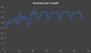
Here’s the result of a run on 1 week of the new data using the incremental algorithm. The best accuracy is 0.72. The x-axis is just the loop number (multiply by 100 to find out how much data has been processed so far). 
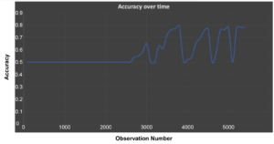
Now compare that to what we observed in the previous blog:
As we saw, the accuracy of incremental learning tends to oscillate wildly, and this run is no exception. Just for comparison, I reran the previous batch training on this data which gave a training accuracy of 0.94, but an evaluation accuracy of less at 0.8 (on 20% of the data).
In the final part of this series, we’ll introduce some concept drift and see how it manages.
