Introduction
There’s no escaping the role that monitoring plays in our everyday lives. Whether it’s from monitoring the weather or the number of steps we take in a day, or computer systems to ever-popular IoT devices.
Practically any activity can be monitored in one form or another these days. This generates increasing amounts of data to be pored over and analyzed–but storing all this data adds significant costs over time. Given this huge amount of data that only increases with each passing day, efficient compression techniques are crucial.
Here at NetApp® Instaclustr we saw a great opportunity to improve the current compression techniques for our time series data. That’s why we created the Advanced Time Series Compressor (ATSC) in partnership with University of Canberra through the OpenSI initiative.
ATSC is a groundbreaking compressor designed to address the challenges of efficiently compressing large volumes of time-series data. Internal test results with production data from our database metrics showed that ATSC would compress, on average of the dataset, ~10x more than LZ4 and ~30x more than the default Prometheus compression. Check out ATSC on GitHub.
There are so many compressors already, so why develop another one?
While other compression methods like LZ4, DoubleDelta, and ZSTD are lossless, most of our timeseries data is already lossy. Timeseries data can be lossy from the beginning due to under-sampling or insufficient data collection, or it can become lossy over time as metrics are rolled over or averaged. Because of this, the idea of a lossy compressor was born.
ATSC is a highly configurable, lossy compressor that leverages the characteristics of time-series data to create function approximations. ATSC finds a fitting function and stores the parametrization of that function—no actual data from the original timeseries is stored. When the data is decompressed, it isn’t identical to the original, but it is still sufficient for the intended use.
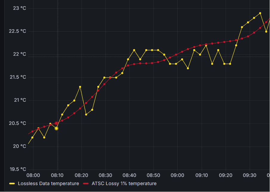
Here’s an example: for a temperature change metric—which mostly varies slowly (as do a lot of system metrics!)—instead of storing all the points that have a small change, we fit a curve (or a line) and store that curve/line achieving significant compression ratios.

Image 1: ATSC data for temperature
How does ATSC work?
ATSC looks at the actual time series, in whole or in parts, to find how to better calculate a function that fits the existing data. For that, a quick statistical analysis is done, but if the results are inconclusive a sample is compressed with all the functions and the best function is selected.
By default, ATSC will segment the data—this guarantees better local fitting, more and smaller computations, and less memory usage. It also ensures that decompression targets a specific block instead of the whole file.
In each fitting frame, ATSC will create a function from a pre-defined set and calculate the parametrization of said function.
ATSC currently uses one (per frame) of those following functions:
- FFT (Fast Fourier Transforms)
- Constant
- Interpolation – Catmull-Rom
- Interpolation – Inverse Distance Weight

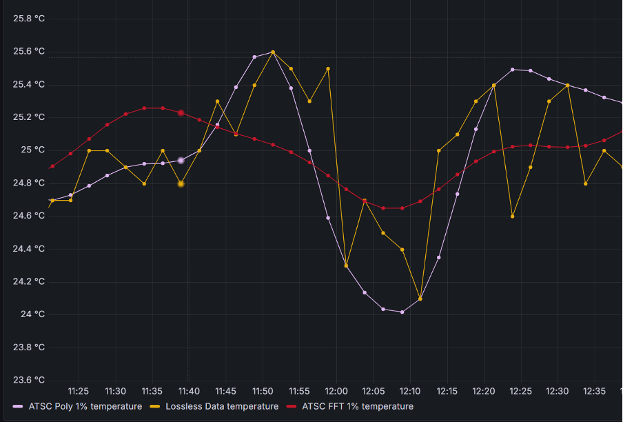
Image 2: Polynomial fitting vs. Fast-Fourier Transform fitting
These methods allow ATSC to compress data with a fitting error within 1% (configurable!) of the original time-series.
For a more detailed insight into ATSC internals and operations check our paper!
Use cases for ATSC and results
ATSC draws inspiration from established compression and signal analysis techniques, achieving compression ratios ranging from 46x to 880x with a fitting error within 1% of the original time-series. In some cases, ATSC can produce highly compressed data without losing any meaningful information, making it a versatile tool for various applications (please see use cases below).
Some results from our internal tests comparing to LZ4 and normal Prometheus compression yielded the following results:
| Method | Compressed size (bytes) | Compression Ratio |
| Prometheus | 454,778,552 | 1.33 |
| LZ4 | 141,347,821 | 4.29 |
| ATSC | 14,276,544 | 42.47 |
Another characteristic is the trade-off between fast compression speed vs. slower compression speed. Compression is about 30x slower than decompression. It is expected that time-series are compressed once but decompressed several times.

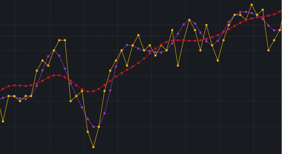
Image 3: A better fitting (purple) vs. a loose fitting (red). Purple takes twice as much space.
ATSC is versatile and can be applied in various scenarios where space reduction is prioritized over absolute precision. Some examples include:
- Rolled-over time series: ATSC can offer significant space savings without meaningful loss in precision, such as metrics data that are rolled over and stored for long term. ATSC provides the same or more space savings but with minimal information loss.
- Under-sampled time series: Increase sample rates without losing space. Systems that have very low sampling rates (30 seconds or more) and as such, it is very difficult to identify actual events. ATSC provides the space savings and keeps the information about the events.
- Long, slow-moving data series: Ideal for patterns that are easy to fit, such as weather data.
- Human visualization: Data meant for human analysis, with minimal impact on accuracy, such as historic views into system metrics (CPU, Memory, Disk, etc.)

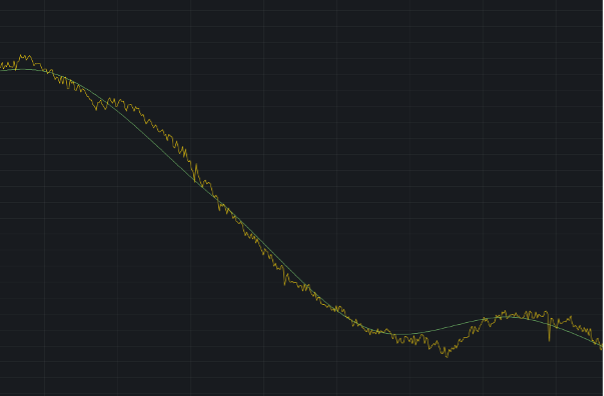
Image 4: ATSC data (green) with an 88x compression vs. the original data (yellow)
Using ATSC
ATSC is written in Rust as and is available in GitHub. You can build and run yourself following these instructions.

Future work
Currently, we are planning to evolve ATSC in two ways (check our open issues):
- Adding features to the core compressor focused on these functionalities:
- Frame expansion for appending new data to existing frames
- Dynamic function loading to add more functions without altering the codebase
- Global and per-frame error storage
- Improved error encoding
- Integrations with additional technologies (e.g. databases):
- We are currently looking into integrating ASTC with ClickHouse® and Apache Cassandra®
|
1 2 3 4 5 6 7 8 9 10 11 12 |
CREATE TABLE sensors_poly ( sensor_id UInt16, location UInt32, timestamp DateTime, pressure Float64 CODEC(ATSC('Polynomial', 1)), temperature Float64 CODEC(ATSC('Polynomial', 1)), ) ENGINE = MergeTree ORDER BY (sensor_id, location, timestamp); |
Image 5: Currently testing ClickHouse integration
Sound interesting? Try it out and let us know what you think.
ATSC represents a significant advancement in time-series data compression, offering high compression ratios with a configurable accuracy loss. Whether for long-term storage or efficient data visualization, ATSC is a powerful open source tool for managing large volumes of time-series data.
But don’t just take our word for it—download and run it!
Check our documentation for any information you need and submit ideas for improvements or issues you find using GitHub issues. We also have easy first issues tagged if you’d like to contribute to the project.
Want to integrate this with another tool? You can build and run our demo integration with ClickHouse.