Introduction: The next phase of Kafka Tiered Storage
In my previous blog series, I explored how Apache Kafka Tiered Storage is more like a dam than a fountain by comparing local vs remote storage (Part 1), performance results (Part 2), Kafka time and space (Part 3), and the impact of various consumer behaviors on the amount and age of data processed (Part 4).
Now that I have a solid understanding of Tiered Storage—it’s a pretty useful feature to have—this did bring up an entirely new set of questions: does my Apache Kafka cluster have to be bigger (and by approximately how much) if I enable Tiered Storage? And what happens if I change producer and/or consumer workloads?
Or, to put it another way: how do you resize a Kafka cluster (using Solid State Drives [SSDs] for local storage) for producer and consumer workloads on topics with remote Tiered Storage enabled?
This new series will explore doing just that by examining the impact of producer and consumer workloads on cluster sizing by using a performance modeling approach.
We’ll then extend the model to include local Elastic Block Store (EBS) storage, take a look at how many brokers (at minimum) are needed, what size AWS instances to use, how big your storage needs to be, and more.
Setting up the model
But first things first: we need to make some assumptions and caveats.
The initial approach for this model will look at the impact of local vs. Tiered Storage for:
- Data workloads only
- Excluding meta-data workloads
- I/O, EBS bandwidth, and network bandwidth only
- CPU demand and utilization is ignored
- Local storage using SSDs (we will compare with EBS storage in the next part)
- The cluster level
- Whole cluster resources rather than brokers or availability zones
- Aggregated/total producer and consumer workloads
- Total producer/consumer workload data bandwidth (in/out) only
- Continuous and average rates
- Ignoring message rates and sizes, the number of topics and partitions
- Assuming no data compression
- Although in practice the model just captures the total volume of data written to and read from the cluster
- Whether it’s compressed or not
- A single cluster
To simplify things even further for this blog, we need a “representative” illustrative cluster.
One of the talks I gave last year was at Community over Code EU (Bratislava); I presented “Why Apache Kafka Clusters Are Like Galaxies (And Other Cosmic Kafka Quandaries Explored)”. Part of this talk was an analysis of performance metrics across our top 10 (biggest) Kafka production clusters.
For this blog, I’m going to use those average metrics, including:
- The average producer input (ingress) bandwidth of 1 GB/s (1,000 MB/s)
- The average fan-out ratio of 3
- i.e. for every byte coming into the cluster, 3 bytes are emitted, implying that there are an average of 3 consumer groups at the cluster level
- Giving an output (egress) bandwidth of 3 GB/s (3,000 MB/s), for our example.
Note that this “average” cluster may not really exist in the top 10 clusters, and we’ll change the assumptions for the fan-out ratio for the last scenario below.
For this blog, I’ve manually built a very simple performance model in Excel and will show the input parameter values and predictions using Sankey Diagrams (which date from the 1800’s when they were first used to show energy flows in steam engines).
I’ve used Sankey diagrams previously to explain system performance to great effect (check out my blogs for Kafka Metrics, OpenTelemetry, and Kafka Kongo).
Why use Sankey Diagrams? Well, because they’re a good choice for performance models as they show values and flows between multiple components on the same diagram. I’ll add one workload type at a time until we complete the model and explore how it works for local vs. remote Tiered Storage, and SSD vs. EBS local storage types.
(Oh, and I’ll do this all with the help of some cheese!)

Cheese is produced from raw ingredients – the first part of its journey to ultimately being consumed… (Source: Adobe Stock)
1. Producers
We’ll start with the basic producer workload, assuming SSD storage for brokers, and that remote Tiered Storage is enabled for all topics.
The following Sankey diagram shows the total producer workload of 1,000 MB/s into the cluster (on the left), resulting in a cluster I/O load (on SSDs) of 1,000 MB/s and network load of 1,000 MB/s (InOutNet).

Basic writes from producers to partition leaders use network bandwidth into the cluster, cluster (local storage) I/O—but no inter broker network or network out of the cluster.
The total of 2,000 MB/s for the ProducersCluster component is a combination of all I/O and Network bandwidth due to the producer workload at the cluster level. For this model at least, it isn’t really a meaningful number at the cluster level, so can just be ignored.
(In practice, however, CPU load is likely to be proportional to the combined I/O and network, and potentially other factors that we haven’t included in the model yet – message rate, number of partitions and consumers, compression, etc.).
The numbers that matter are on the left and right-hand sides.

…and after production, cheese is then replicated… (Source: Adobe Stock)
2. Replication
Next, we add the replication workload due to the producer workload.
This workload copies records from the leader partitions (from active segments, assumed to be in the cache so there’s no I/O local on the leaders), to the follower brokers (with RF=3 the number of followers = 2). This contributes double (x2) of the producer input bandwidth (1,000 x 2 = 2,000 MB/s to both the cluster network (broker to broker) and local I/O, taking the total I/O and network bandwidth to 3,000 MB/s.

Leader partition replication copies from the cache on the leader broker to the number of followers (2 for RF=3) using cluster network and I/O to write on each follower.

…and then stored remotely (even in caves)… (Source: Adobe Stock)
3. Remote Tiered Storage writes
With remote storage enabled (we assume for all topics), closed segments are copied to remote storage—the reading of this data uses cluster I/O (for SSDs) and network for transferring it to remote cloud storage (e.g. AWS S3).
We assume that closed segments are no longer in the cache so must use I/O to read from local storage (i.e. there is a delay between records being written to the active segment, and the active segment being eventually closed and asynchronous copying of the records to remote storage).
The next diagram adds the remote storage writes workload including the reads from local storage (I/O, 1,000 MB/s), and writes to remote storage using the network (1,000 MB/s), this takes the combined I/O load to 4,000 MB/s and combined network load to 4,000 MB/s.
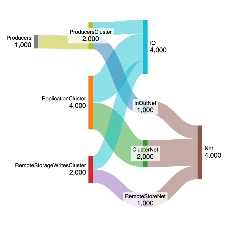
Note that the remote storage workload is comparable to adding a delayed-consumer (see below) in terms of the overhead on I/O and network.
So even with an incomplete model, what can tell about the overhead of Tiered Storage for the write workloads? Comparing the load predicted by this diagram with the previous one we can see that for writes there’s about a 25% overhead for Tiered Storage. For a 1GB/s producer workload, and all topics enabled for Tiered Storage: 4,000 MB/s I/O and network for Tiered Storage, c.f. 3,000 MB/s I/O and network for local storage.
So, what happens when we add consumer workloads? Bring on the mice!

…and then ultimately consumed! (Source: Adobe Stock)
4. Consumer workloads
For simplicity, we model consumer workloads as a combination of real-time, delayed or remote. Given the fan-out of 3 for this representative cluster, we assume an initial ratio of 100%:100%:100% across the different consumer workloads (1,000 MB/s per consumer type, a total of 3,000 MB/s).
Real-time consumers are assumed to keep up with the producer rates, so read from local cache only. They use 1,000 MB/s of network only.
Delayed consumers are assumed to be running a bit behind the producers, so are likely to read from local storage. They use 1,000 MB/s each of I/O and Network.
Remote consumers may re-read from the start of topics and are assumed to use remote storage only. They use 2,000 MB/s of network in total (1,000 MB/s with the broker, and 1,000 MB/s with the remote storage).
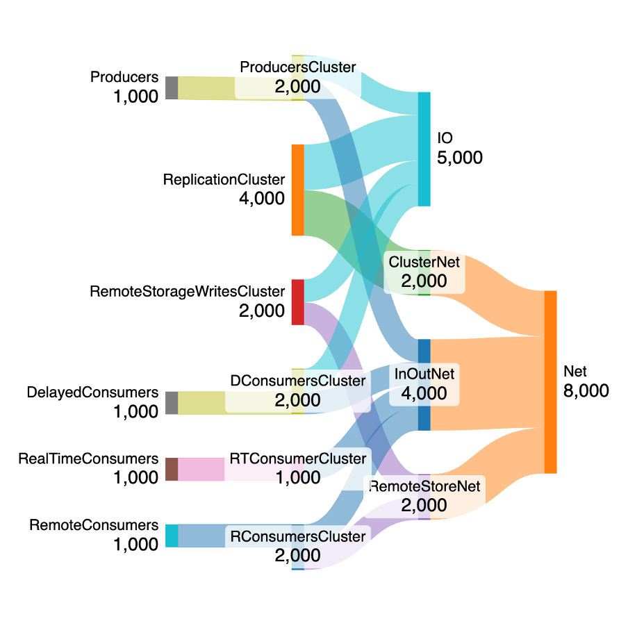
This gives a grand total of 5,000 MB/s for I/O, and 8,000 MB/s for network bandwidth used for Tiered Storage enabled for this scenario. I used SankeyMATIC, and below is an example model, so you can copy it to https://sankeymatic.com/build/ and try it yourself.
// Tiered Storage, SSDs
// producer workload, 1,000 MB/s in
Producers [1000] ProducersCluster
ProducersCluster [1000] IO
ProducersCluster [1000] InOutNet
// producer RF workload, RF=3 so x2 producer workload
ReplicationCluster [2000] IO
ReplicationCluster [2000] ClusterNet
// remote storage workload, copies from local storage to remote storage
RemoteStorageWritesCluster [1000] IO
RemoteStorageWritesCluster [1000] RemoteStoreNet
RealTimeConsumers [1000] RTConsumerCluster
RTConsumerCluster [1000] InOutNet
DelayedConsumers [1000] DConsumersCluster
DConsumersCluster [1000] IO
DConsumersCluster [1000] InOutNet
RemoteConsumers [1000] RConsumersCluster
RConsumersCluster [1000] InOutNet
RConsumersCluster [1000] RemoteStoreNet
// Total Network is sum of In/Out, Cluster and Remote network
InOutNet [4000] Net
ClusterNet [2000] Net
RemoteStoreNet [2000] Net

Cheese (like clusters) comes in different sizes (Source: Adobe Stock)
5. Local vs. remote storage sizing
Now that we have a complete model of remote storage, we can compare this with a complete model of local storage and see what the size difference is likely to be.
For local-only storage, there are no remote workloads (writes to remote storage, or consumers from remote storage), and we assume a 50/50 split of real-time and delayed consumers and fan-out of 3 still (i.e. the total consumer workload is still 1,500 + 1,500 = 3,000 MB/s but split across two not three workload types as in the remote storage model). Here’s the local storage model:

What overhead is there for Tiered Storage for this scenario? The following graph shows the comparison between network (5,000/8,000 MBs) and I/O (4,500/6,000 MBs) for local vs. remote storage, revealing an overhead of 33% for Network and 11% for I/O.

6. Scaling the remote consumer workload
As I mentioned in the introduction, the “average” cluster may not in fact exist in our top 10 clusters, and there is a significant variation in workloads and cluster sizes across the top 10.
Having a Kafka cluster with remote storage enabled and lots of records stored on cloud native storage opens up the possibilities for new consumer workload use cases, including replaying and reprocessing a larger number of historical records, or migrating all the records to a new sink system, etc.
In common with the delayed consumer workload in our model, the remote consumer workload is also not limited to the incoming producer rate—it can in theory be faster. Let’s explore what happens when the remote consumer workload rate is significantly higher.
Let’s assume a similar real-time consumer workload as the local scenario above, but no delayed workload. In theory, with remote storage, you could reduce the local retention rate and therefore the size of local storage (SSDs in this case) to close to zero and rely entirely on the remote storage for processing older records.
Let’s therefore increase the remote consumer workload rate substantially to 10,000 MB/s (x10 the producer input rate). As there is a lot of data in remote storage it will take longer to read and process than the original producer/real-time workloads, so this assumption is more realistic for processing lots of historical data. This gives a fan-out ratio of 11.5.
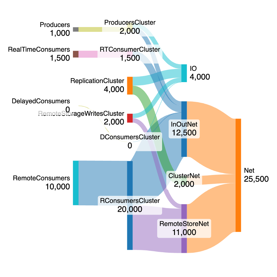
The network load rate has jumped substantially to 25,500 MB/s, around 3x the original default Tiered Storage scenario network usage or 4x the local only scenario. This is logical, as increasing the remote consumer workload will result in more network load (as the read path is consumer → broker → remote storage). And more CPU will also be needed.

Apache Kafka can sometimes be…Kafkaesque! (Source: Bing AI Generated)
7. Scaling in practice
But watch out! To significantly increase the remote consumer workload throughput, you need to have previously increased the number of topic partitions—in fact, before the data was written to remote storage.
This is because for higher consumer concurrency you need more consumers and partitions, and even though remote storage doesn’t “use” partitions, it only stores the data as it existed on local storage initially— i.e. with the partitions that originally existed.
So, increasing the number of consumers before reading back to more than the number of partitions that the remote storage segments were written with won’t increase the read concurrency—it will just mean some consumers time out due to read starvation.
However, it will work if there are sufficient partitions in the original data, sufficient consumers and consumer resources, and importantly, as long as there are sufficient cluster resources including CPU and network.
Note that this partition constraint is common to all consumer workload types (real-time and delayed). The difference is that cloud-native storage such as AWS S3 is elastic and scalable; if the load increases gradually, in the same region and with sufficient connections and error handling. On the other hand, SSDs have fixed non-elastic I/O limits (although real-time consumer workloads are likely faster due to reading directly from the kernel page cache).
Also, remember that consuming from remote storage will increase read latencies (see Part 2 of my Kafka Tiered Storage series) which will necessitate an increase in the number of partitions and consumers to achieve higher throughput.
And if you are using Kafka® Connect for a scenario like migrating data from an existing Kafka cluster to a new sink system, then you may need a bigger Kafka Connect cluster, more connector workers/tasks, and to check that the sink system can cope with the expected load.
For more about scaling Kafka Connect, check out my real-time zero-code data pipeline series here.
Conclusion and what’s next
By leveraging performance models and diagrams, we’ve successfully compared local and remote storage setups, showcasing the trade-offs in scalability and resource usage. Scaling workloads, particularly for remote consumers accessing historical data, emphasizes the importance of planning partitions and cluster resources.
That’s all for now! In the next part of this series, we’ll explore a Kafka Tiered Storage model using AWS EBS for local storage (c.f. SSD), and more.
This is the first part in my new series on sizing clusters for Kafka Tiered Storage. Check out my companion series exploring Tiered Storage from the ground up–and why it’s more like a dam than a fountain!
Part 1: Introduction to Kafka Tiered Storage
Part 2: Tiered Storage performance
Part 4: Tiered Storage use cases
Want to create a NetApp Instaclustr Apache Kafka cluster with Tiered Storage? See our support documentation Using Kafka Tiered Storage. We recently added new metrics for Tiered Storage clusters, making the feature even cooler!
Try it out yourself and spin up your first cluster on the Instaclustr Managed Platform with a free no-obligation 30-day trial of developer-sized instances.
Update!
I’ve put some of the functionality from the Excel model into a prototype JavaScript/HTML Kafka sizing calculator available from GitHub. This includes EBS modelling which you can read about in the next blog.